Change Point Regression

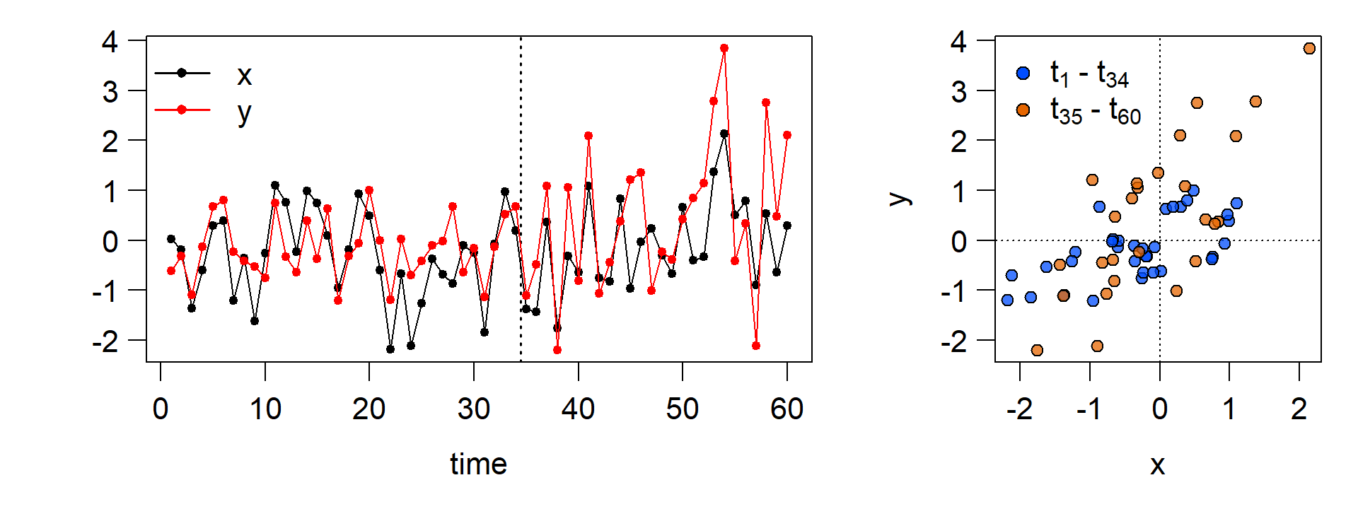
The regression model

Now we build a model that can recover the change point and the linear relationship between $x$ and $y$ before and after the change point.

The first part of this model looks like an ordinary least squares regression of $y$ against $x$:

$\begin{array}{r}\begin{array}{l}{y}_i\sim N({\mu }_i,{\sigma }_1^2),\\ {\mu }_i={\alpha }_1+{\beta }_1{x}_i,i=1,...,n_{change}-1\end{array}\end{array}$

Here we have a single intercept (${\alpha }_1$), slope (${\beta }_1$), and residual variance (${\sigma }_1^2$). $n_{change}$ - 1 denotes the number of obervations before the change point.

From the change point $n_{change}$ onwards, we add an additional intercept, ${\alpha }_2$, to the intercept from the first part (${\alpha }_1$). We do the same for the slope and the residual variance:

$\begin{array}{r}\begin{array}{l}{y}_i\sim N({\mu }_i,{\sigma }_1^2+{\sigma }_2^2),\\ {\mu }_i={\alpha }_1+{\alpha }_2+({\beta }_1+{\beta }_2)x_i,i=n_{change},...,n\end{array}\end{array}$

$n$ denotes the total number of observations, 60 in this case. But how do we actually find the change point $n_{change}$?

Implementation in JAGS

Here, we turn to the JAGS programming environment. Understanding a model written for JAGS is not easy at first. If you are keen on learning Bayesian modeling from scratch I can highly recommend Richard McElreath’s book Statistical Rethinking. We will access JAGS with the R2jags package, so we can keep using R even if we are writing a model for JAGS.

Bayesian methods for detecting change points are also available in Stan, as discussed here. An application using English league football data can be found here.

Below, we look at the model. The R code that will be passed to JAGS later is on the left. On the right is an explanation for each line of the model.

model_CPR <- function(){
  
  ### Likelihood or data model part
  for(i in 1:n){
    
  y[i] ~ dnorm(mu[i], tau[i]) 

    
    
  mu[i] <- alpha_1 + 
  alpha_2 * step(i - n_change) +
  (beta_1 + beta_2 * step(i - n_change))*x[i]
  
  
  
  tau[i] <- exp(log_tau[i])
  
  log_tau[i] <- log_tau_1 + log_tau_2 * 
  step(i - n_change)
  } 
  
  ### Priors
  
  
  alpha_1 ~ dnorm(0, 1.0E-4)
  
  
  alpha_2 ~ dnorm(0, 1.0E-4)
  
  beta_1 ~ dnorm(0, 1.0E-4)
  beta_2 ~ dnorm(0, 1.0E-4)
  
  log_tau_1 ~ dnorm(0, 1.0E-4)
  log_tau_2 ~ dnorm(0, 1.0E-4)
  
  K ~ dcat(p)
  n_change <- possible_change_points[K]

}

Note that we put priors on $\log ({\tau }_1)$ and $\log ({\tau }_2)$, rather than on ${\tau }_1$ and ${\tau }_2$ directly, to ensure that the precision $\tau$ in the second part of the regression always remains positive. $e^{\log ({\tau }_1)+\log ({\tau }_2)}$ is always $>0$, even if the term $\log ({\tau }_1)$ + $\log ({\tau }_2)$ becomes negative.

Prepare the data which we pass to JAGS along with the model:

# minimum number of the data points before and after the change
  min_segment_length <- 5 

# assign indices to the potential change points we allow
  possible_change_points <- (1:n)[(min_segment_length+1):(n+1-min_segment_length)] 
 
# number of possible change points
  M <- length(possible_change_points)  

# probabilities for the discrete uniform prior on the possible change points, 
# i.e. all possible change points have the same prior probability
  p <- rep(1 / M, length = M) 
 
# save the data to a list for jags
  data_CPR <- list("x", "y", "n", "possible_change_points", "p") 

Load the R2jags package to access JAGS in R:

  library(R2jags) 

Now we execute the change point regression. We instruct JAGS to run three seperate chains so we can verify that the results are consistent. We allow 2000 iterations of the Markov chain Monte Carlo algorithm for each chain, the first 1000 of which will automatically be discarded as burn-in.

 CPR  <- jags(data = data_CPR, 
                         parameters.to.save = c("alpha_1", "alpha_2", 
                                                "beta_1","beta_2",
                                                "log_tau_1","log_tau_2",
                                                "n_change"), 
                         n.iter = 2000, 
                         n.chains = 3,
                         model.file = model_CPR)

The results

To visualise the results and inspect the posterior, we are using the ggmcmc package, which relies on the ggplot2 package. For brevity, we just look at the $n_{change}$ parameter here.

library(ggmcmc)
CPR.ggs <- ggs(as.mcmc(CPR)) # convert to ggs object
ggs_traceplot(CPR.ggs, family = "n_change")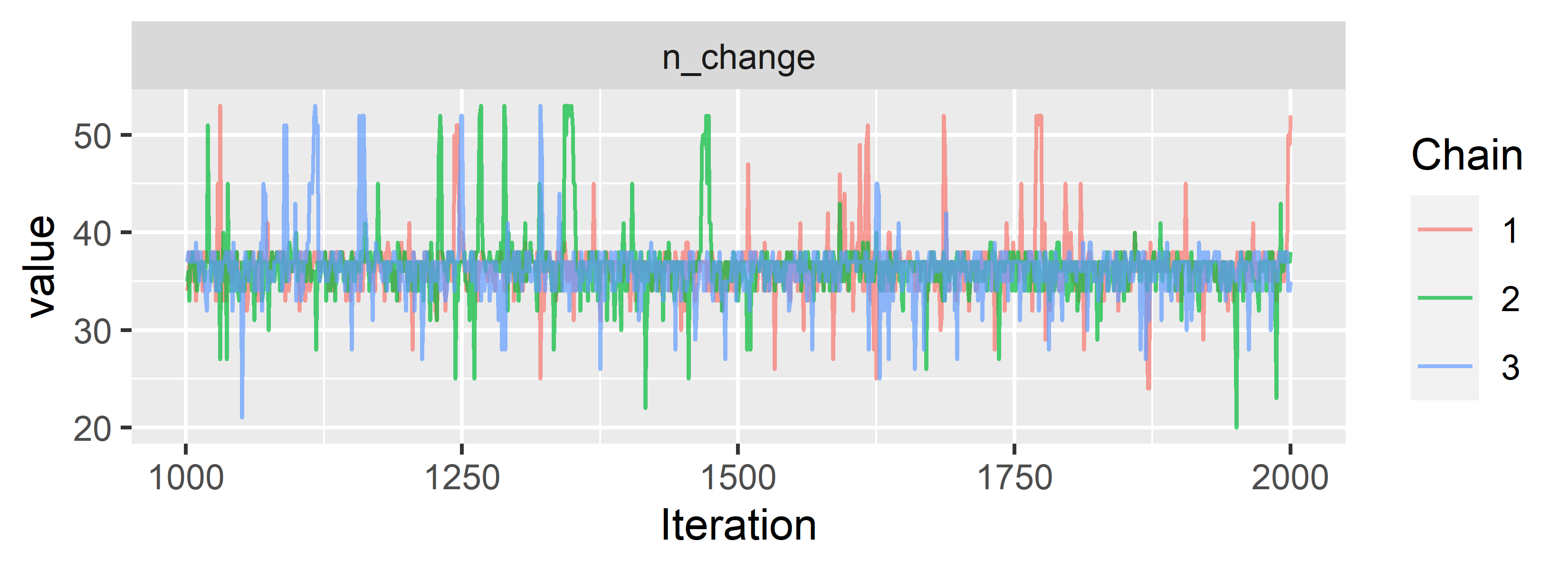 

Looks like the chains converge and mix nicely. We can already see that our model locates the change point somewhere between $30$ and $40$, although the chains occasionally explore regions further away.

Let’s look at the posterior probabilities for the possible change points:

ggplot(data = CPR.ggs %>% filter(Parameter == "n_change"),
  aes(x=value, y = 3*(..count..)/sum(..count..), fill = as.factor(Chain))) + 
  geom_vline(xintercept = 35,lty = 2) + geom_bar(position = "identity", alpha = 0.5) +
  ylab("posterior probability") + xlab("n_change") + labs(fill='Chain')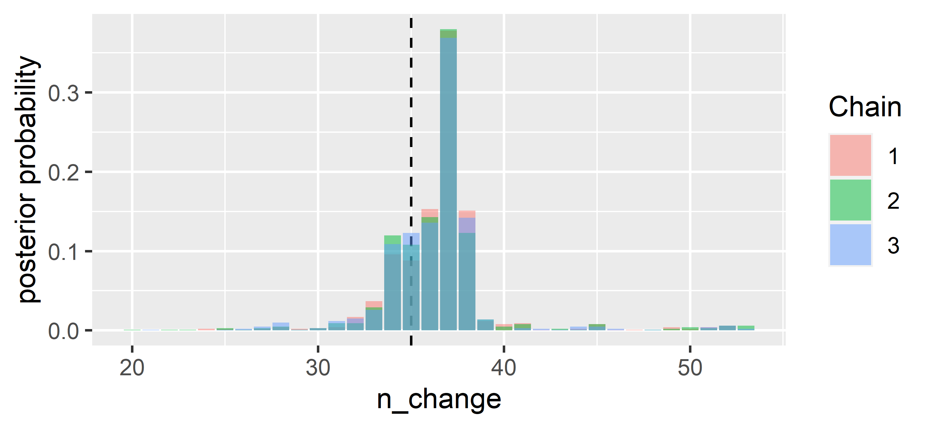

The ${37}^{th}$ point has the highest probability of being the change point. That is not far off from where we introduced the change, at the ${35}^{th}$ point (dashed line). The random generation of $x$ and $y$ has led to $37$ being favoured. We also note that there are only minor differences between the three chains, and those differences would likely further dwindle if we were to let the chains run for longer.

Using the posterior distribution, we can answer questions like: “In which interval does the change point fall with 90 % probability?”

quantile(CPR$BUGSoutput$sims.list$n_change, probs = c(0.05, 0.95))

##  5% 95% 
##  33  39

We can also inquire about the probability that the change point falls in the interval $34$ to $38$:

round(length(which(CPR$BUGSoutput$sims.list$n_change %in% 34:38))/
              (CPR$BUGSoutput$n.sims),2)

## [1] 0.87

Finally, let’s have a look at the regression parameters and plot the resulting regressions before and after the most likely change point.

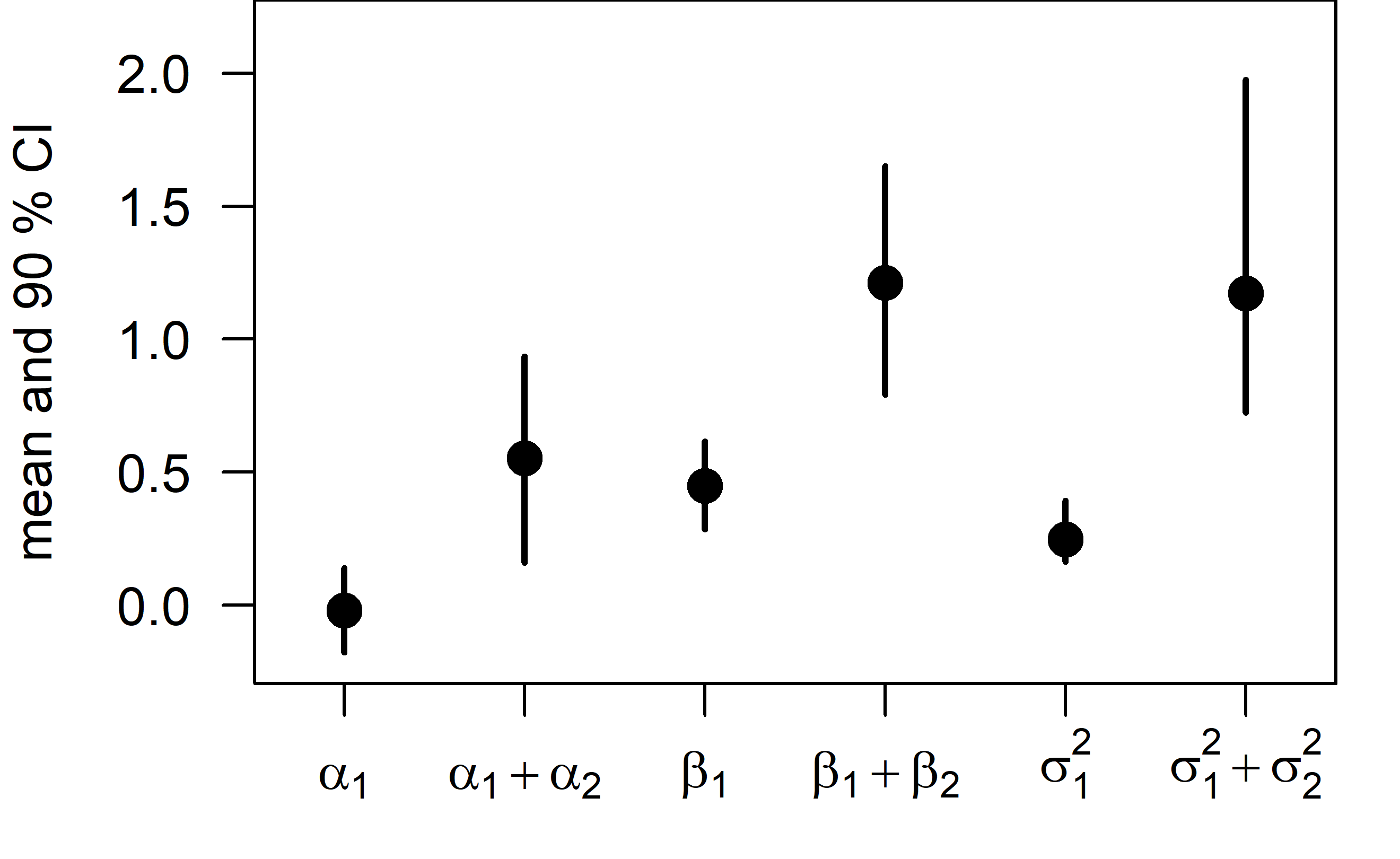The intercept, slope, and residual variance all increase after the change point.

This can be immediately seen when plotting the change point regression: 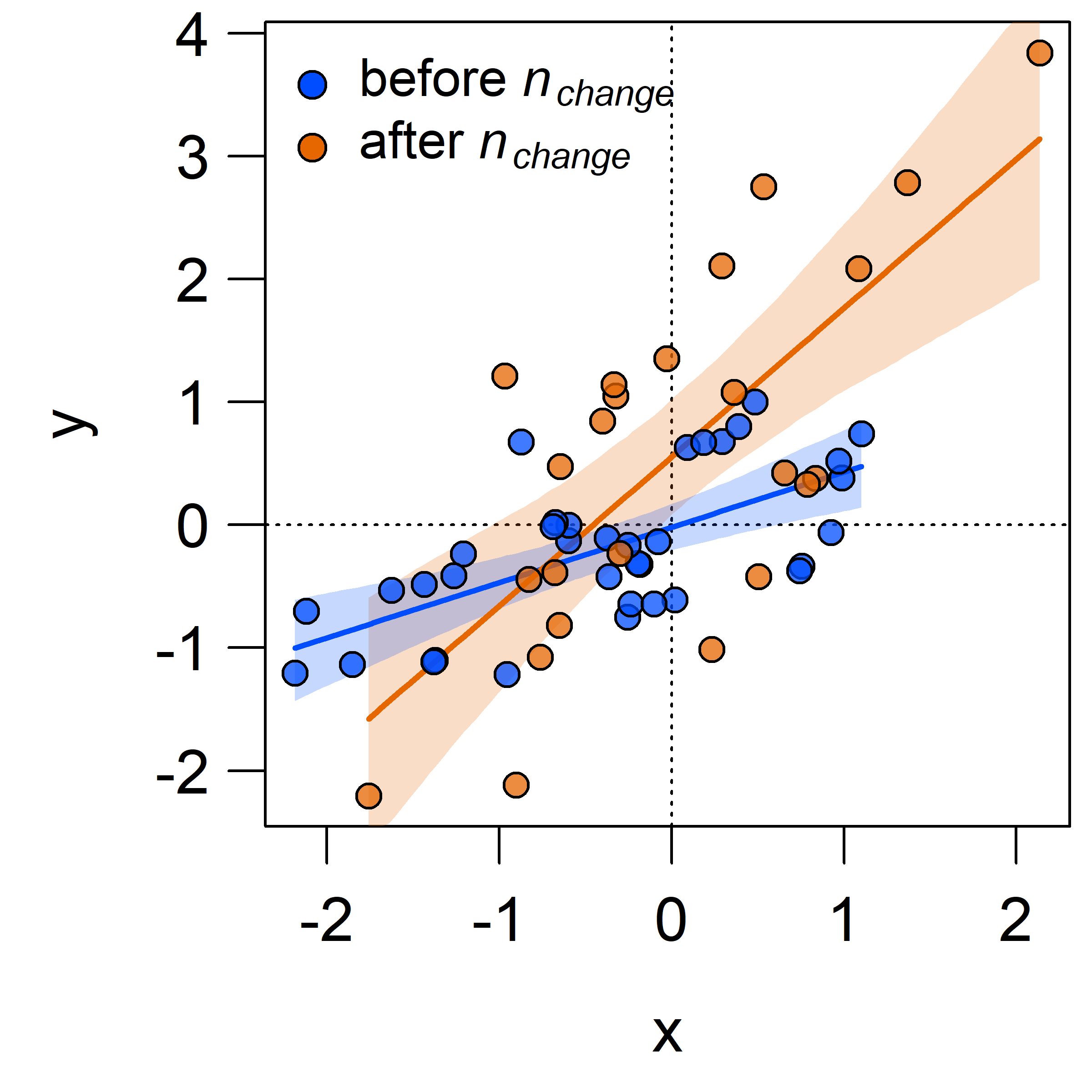The shaded areas denote $95$ % credible intervals around the regression lines.

You can find the full R code for this analysis at https://github.com/KEichenseer/Bayesian-Models/blob/main/01-Change_point_regression_with_JAGS.R

Get in touch if you have any comments or questions!